Akida user guide

Overview

Like many other machine learning frameworks, the core data structures of Akida are layers and models, and users familiar with Keras, Tensorflow or Pytorch should be on familiar ground.

The main difference between Akida and other machine learning networks is that inputs and weights are integers and it only performs integer operations, so that it can further reduce the power consumption and memory footprint. Since quantization and ReLU activation functions lead to a substantial sparsity, Akida takes advantage of this by implementing operations in biologically inspired event-based calculations. However, to simplify the user experience, the model weights and the inputs are represented as integer tensors (Numpy arrays), similar to what you would see in other machine learning frameworks.

Going from the standard deep learning world to Akida world is done by following simple steps:

• build a model using Keras or optionally using a model from the Brainchip zoo

• quantize the model using the QuantizeML toolkit

• convert the model to Akida using the CNN2SNN toolkit

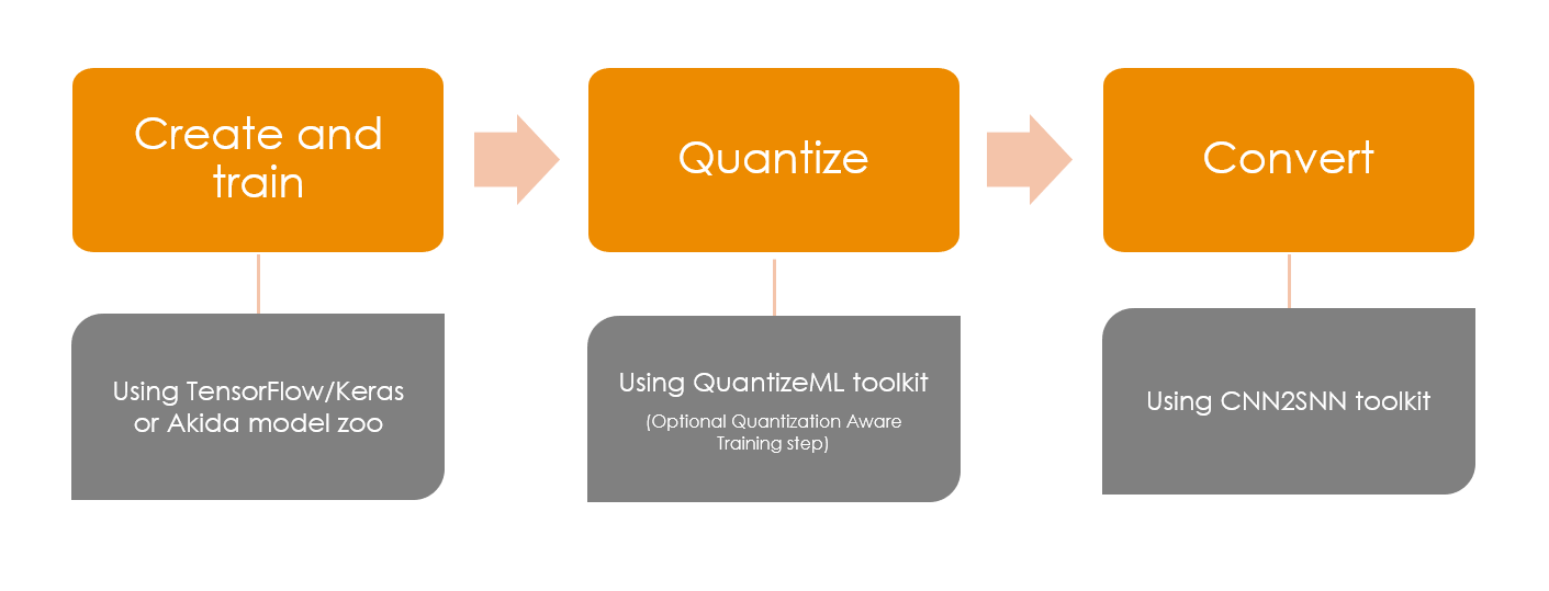
Akida workflow

A practical example of the overall flow is given in the examples section, see the workflow tutorial.

Programming interface

The Akida Model

Similar to other deep learning frameworks, Akida offers a Model grouping layers into an object with inference features.

The Model object has basic features such as:

• summary() method that prints a description of the model architecture.

• save() method that needs a path for the model and that allows saving to disk for future use. The model will be saved as a file with an .fbz extension. A saved model can be reloaded using the Model object constructor with the full path of the saved file as a string argument. This will automatically load the model weights.

  from akida import Model
  
  model.save("my_model.fbz")
  loaded_model = Model("my_model.fbz")
  

• forward method to generate the outputs for a specific set of inputs.

  import numpy as np
  
  # Prepare one sample
  input_shape = (1,) + tuple(model.input_shape)
  inputs = np.ones(input_shape, dtype=np.uint8)
  # Inference
  outputs = model.forward(inputs)
  

• predict method is very similar to the forward method, but is specifically designed to replicate the float outputs of a converted CNN.

• statistics member provides relevant inference statistics.

Akida layers

The sections below list the available layers for Akida 1.0 and Akida 2.0. Those layers are obtained from converting a quantized model to Akida and are thus automatically defined during conversion. Akida layers only perform integer operations using 8-bit or 4-bit quantized inputs and weights. The exception is FullyConnected layers performing edge learning, where both inputs and weights are 1-bit.

Akida 1.0 layers

• InputData

• InputConvolutional

• FullyConnected

• Convolutional

• SeparableConvolutional

Akida 2.0 layers

• InputData

• InputConv2D

• Stem

• Conv2D

• Conv2DTranspose

• Dense1D

• Dense2D

• DepthwiseConv2D

• DepthwiseConv2DTranspose

• Attention

• Add

• Concatenate

• ExtractToken

• BatchNormalization

• MadNorm

• Shiftmax

• Dequantizer

Model Hardware Mapping

By default, Akida models are implicitly mapped on a software backend: in other words, their inference is computed on the host CPU.

Devices

In order to perform model inference on hardware, the corresponding Model object must first be mapped on a specific Device.

The Akida Device represents a device object that holds a version and the hardware topology of the mesh. The main properties of such object are:

• its hardware version,

• the description of its mesh of processing nodes.

Discovering Hardware Devices

The list of hardware devices detected on a specific host is available using the devices() method.

from akida import devices

device = devices()[0]
print(device.version)

It is also possible to list the available devices using a command in a terminal:

akida devices

Virtual Devices

Most of the time, Device objects are real hardware devices, but virtual devices can also be created to allow the mapping of a Model on a host that is not connected to a hardware device.

It is possible to build a virtual device for known hardware devices, by calling functions AKD1000() and TwoNodesIP().

Model mapping

Mapping a model on a specific device is as simple as calling the Model .map() method.

model.map(device)

When mapping a model on a device, if the Model is too big to fit on the device or contains layers that are not hardware compatible, it will be split into multiple parts called “sequences”.

The number of sequences, program size for each and how they are mapped are included in the Model .summary() output after it has been mapped on a device.

Advanced Mapping Details and Hardware Devices Usage

When Model .map() results in more than one hardware sequence, on inference each sequence will be chain loaded onto the device to process a given input. Sequences can be obtained using the Model .sequences() property, that will return a list of sequence objects. The program used to load one sequence can be obtained programmatically.

model.map(device)
print(len(model.sequences))
# Assume there is at least one sequence.
sequence = model.sequences[0]
# Check program size
print(len(sequence.program))

Once the model has been mapped, the sequences mapped in the Hardware run on the device, and the sequences mapped in the Software run on the CPU.

Note

Where mapping to a single on-hardware sequence is necessary, one can force an exception to be raised if that fails by setting the hw_only parameter to True (default False). See the .map() method API for more details.

model.map(device, hw_only=True)

Once the model has been mapped, the inference happens only on the device, and not on the host CPU except for passing inputs and fetching outputs.

Performance measurement

Performance measures (FPS and power) are available for on-device inference.

Enabling power measurement is simply done by:

device.soc.power_measurement_enabled = True

After sending data for inference, performance measurements can be retrieved from the model statistics.

model_akida.forward(data)
print(model_akida.statistics)

An example of power and FPS measurements is given in the AkidaNet/ImageNet tutorial.

Using Akida Edge learning

Akida Edge learning is a unique feature of the Akida IP, whereby a classifier layer is enabled for ongoing (“continual”) learning in the on-device setting, allowing the addition of new classes in the wild. As with any transfer learning or domain adaptation task, best results will be obtained if the Akida Edge layer is added as the final layer of a standard pretrained CNN backbone. An unusual aspect is that the backbone needs an extra layer added and trained, to generate binary inputs to the Edge layer.

In this mode, an Akida Layer will typically be compiled with specific learning parameters and then undergo a period of feed-forward unsupervised or semi-supervised training by letting it process inputs generated by previous layers from a relevant dataset.

Once a layer has been compiled, new learning episodes can be resumed at any time, even after the model has been saved and reloaded.

Learning constraints

Only the last layer of a model can be trained with Akida Edge Learning and must fulfill the following constraints:

• must be of type FullyConnected,

• must have binary weight,

• must receive binary inputs.

Note

• a FullyConnected layer can only be added to a model defined using Akida 1.0 layers

• it is only possible to obtain a FullyConnected layer from conversion when target version is set to AkidaVersion.v1

Compiling a layer

For a layer to learn using Akida Edge Learning, it must first be compiled using the Model .compile method.

There is only one optimizer available for the compile method which is AkidaUnsupervised and it offers the following learning parameters that can be specified when compiling a layer:

• num_weights: integer value which defines the number of connections for each neuron and is constant across neurons. When determining a value for num_weights note that the total number of available connections for a Convolutional layer is not set by the dimensions of the input to the layer, but by the dimensions of the kernel. Total connections = kernel_size x num_features, where num_features is typically the filters or units of the preceding layer. num_weights should be much smaller than this value – not more than half, and often much less.

• [optional] num_classes: integer value, representing the number of classes in the dataset. Defining this value sets the learning to a ‘labeled’ mode, when the layer is initialized. The neurons are divided into groups of equal size, one for each input data class. When an input packet is sent with a label included, only the neurons corresponding to that input class are allowed to learn.

• [optional] initial_plasticity: floating point value, range 0–1 inclusive (defaults to 1). It defines the initial plasticity of each neuron’s connections or how easily the weights will change when learning occurs; similar in some ways to a learning rate. Typically, this can be set to 1, especially if the model is initialized with random weights. Plasticity can only decrease over time, never increase; if set to 0 learning will never occur in the model.

• [optional] min_plasticity: floating point value, range 0–1 inclusive (defaults to 0.1). It defines the minimum level to which plasticity will decay.

• [optional] plasticity_decay: floating point value, range 0–1 inclusive (defaults to 0.25). It defines the decay of plasticity with each learning step, relative to the initial_plasticity.

• [optional] learning_competition: floating point value, range 0–1 inclusive (defaults to 0). It controls competition between neurons. This is a rather subtle parameter since there is always substantial competition in learning between neurons. This parameter controls the competition from neurons that have already learned – when set to zero, a neuron that has already learned a given feature will not prevent other neurons from learning similar features. As learning_competition increases such neurons will exert more competition. This parameter can, however, have serious unintended consequences for learning stability; we recommend that it should be kept low, and probably never exceed 0.5.

The only mandatory parameter is the number of active (non-zero) connections that each of the layer neurons has with the previous layer, expressed as the number of active weights for each neuron.

Optimizing this value is key to achieving high accuracy in the Akida NSoC. Broadly speaking, the number of weights should be related to the number of events expected to compose the items’ or item’s sub-features of interest.

Tips to set Akida learning parameters are detailed in the dedicated example.