Note
Go to the end to download the full example code.
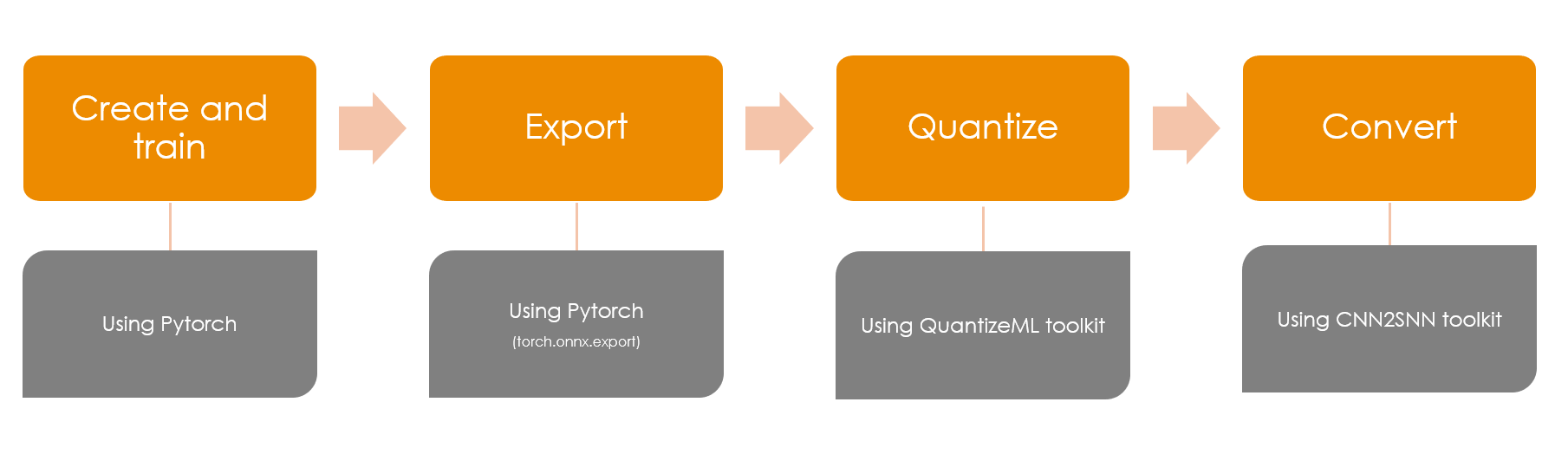
PyTorch to Akida workflow
The Global Akida workflow guide describes the steps to prepare a model for Akida starting from a TensorFlow/Keras model. Here we will instead describe a workflow to go from a model trained in PyTorch.
Note
QuantizeML natively allows the quantization and fine-tuning of TensorFlow models. While it does not support PyTorch quantization natively, it allows to quantize float models stored in the Open Neural Network eXchange (ONNX) format. Export from PyTorch to ONNX is well supported, and so this provides a straightforward pathway to prepare your PyTorch model for Akida.
As a concrete example, we will prepare a PyTorch model on a simple classification task (MNIST). This model will then be exported to ONNX and quantized to 8-bit using QuantizeML. The quantized model is then converted to Akida, and performance evaluated to show that there has been no loss in accuracy.
Please refer to the Akida user guide for further information.
Note
pip install torch==2.0.1 torchvision
Warning
PyTorch Akida workflow
1. Create and train
1.1. Load and normalize MNIST dataset
import torch
import torchvision
import torchvision.transforms as transforms

import matplotlib.pyplot as plt

batch_size = 128


def get_dataloader(train, batch_size, num_workers=2):
    transform = transforms.Compose([transforms.ToTensor(),
                                    transforms.Normalize(0.5, 0.5)])
    dataset = torchvision.datasets.MNIST(root='datasets/mnist',
                                         train=train,
                                         download=True,
                                         transform=transform)
    return torch.utils.data.DataLoader(dataset,
                                       batch_size=batch_size,
                                       shuffle=train,
                                       num_workers=num_workers)


# Load MNIST dataset and normalize between [-1, 1]
trainloader = get_dataloader(train=True, batch_size=batch_size)
testloader = get_dataloader(train=False, batch_size=batch_size)


def imshow(img):
    # Unnormalize
    img = img / 2 + 0.5
    npimg = img.numpy()
    plt.imshow(npimg.transpose((1, 2, 0)))
    plt.show()


# Get some random training images
images, labels = next(iter(trainloader))
Downloading http://yann.lecun.com/exdb/mnist/train-images-idx3-ubyte.gz
Failed to download (trying next):
HTTP Error 403: Forbidden

Downloading https://ossci-datasets.s3.amazonaws.com/mnist/train-images-idx3-ubyte.gz
Downloading https://ossci-datasets.s3.amazonaws.com/mnist/train-images-idx3-ubyte.gz to datasets/mnist/MNIST/raw/train-images-idx3-ubyte.gz

  0%|          | 0/9912422 [00:00<?, ?it/s]
  1%|          | 98304/9912422 [00:00<00:18, 530350.64it/s]
  4%|▍         | 393216/9912422 [00:00<00:08, 1157214.38it/s]
 10%|█         | 1015808/9912422 [00:00<00:03, 2737629.99it/s]
 23%|██▎       | 2293760/9912422 [00:00<00:01, 5824208.68it/s]
 30%|███       | 3014656/9912422 [00:00<00:01, 4727670.62it/s]
 63%|██████▎   | 6258688/9912422 [00:00<00:00, 11589816.55it/s]
 78%|███████▊  | 7766016/9912422 [00:01<00:00, 10047366.52it/s]
100%|██████████| 9912422/9912422 [00:01<00:00, 8517134.61it/s]
Extracting datasets/mnist/MNIST/raw/train-images-idx3-ubyte.gz to datasets/mnist/MNIST/raw

Downloading http://yann.lecun.com/exdb/mnist/train-labels-idx1-ubyte.gz
Failed to download (trying next):
HTTP Error 403: Forbidden

Downloading https://ossci-datasets.s3.amazonaws.com/mnist/train-labels-idx1-ubyte.gz
Downloading https://ossci-datasets.s3.amazonaws.com/mnist/train-labels-idx1-ubyte.gz to datasets/mnist/MNIST/raw/train-labels-idx1-ubyte.gz

  0%|          | 0/28881 [00:00<?, ?it/s]
100%|██████████| 28881/28881 [00:00<00:00, 319358.03it/s]
Extracting datasets/mnist/MNIST/raw/train-labels-idx1-ubyte.gz to datasets/mnist/MNIST/raw

Downloading http://yann.lecun.com/exdb/mnist/t10k-images-idx3-ubyte.gz
Failed to download (trying next):
HTTP Error 403: Forbidden

Downloading https://ossci-datasets.s3.amazonaws.com/mnist/t10k-images-idx3-ubyte.gz
Downloading https://ossci-datasets.s3.amazonaws.com/mnist/t10k-images-idx3-ubyte.gz to datasets/mnist/MNIST/raw/t10k-images-idx3-ubyte.gz

  0%|          | 0/1648877 [00:00<?, ?it/s]
  6%|▌         | 98304/1648877 [00:00<00:02, 531552.62it/s]
 22%|██▏       | 360448/1648877 [00:00<00:01, 1046929.01it/s]
 48%|████▊     | 786432/1648877 [00:00<00:00, 2040914.54it/s]
 97%|█████████▋| 1605632/1648877 [00:00<00:00, 3922658.08it/s]
100%|██████████| 1648877/1648877 [00:00<00:00, 2874590.65it/s]
Extracting datasets/mnist/MNIST/raw/t10k-images-idx3-ubyte.gz to datasets/mnist/MNIST/raw

Downloading http://yann.lecun.com/exdb/mnist/t10k-labels-idx1-ubyte.gz
Failed to download (trying next):
HTTP Error 403: Forbidden

Downloading https://ossci-datasets.s3.amazonaws.com/mnist/t10k-labels-idx1-ubyte.gz
Downloading https://ossci-datasets.s3.amazonaws.com/mnist/t10k-labels-idx1-ubyte.gz to datasets/mnist/MNIST/raw/t10k-labels-idx1-ubyte.gz

  0%|          | 0/4542 [00:00<?, ?it/s]
100%|██████████| 4542/4542 [00:00<00:00, 8137773.93it/s]
Extracting datasets/mnist/MNIST/raw/t10k-labels-idx1-ubyte.gz to datasets/mnist/MNIST/raw
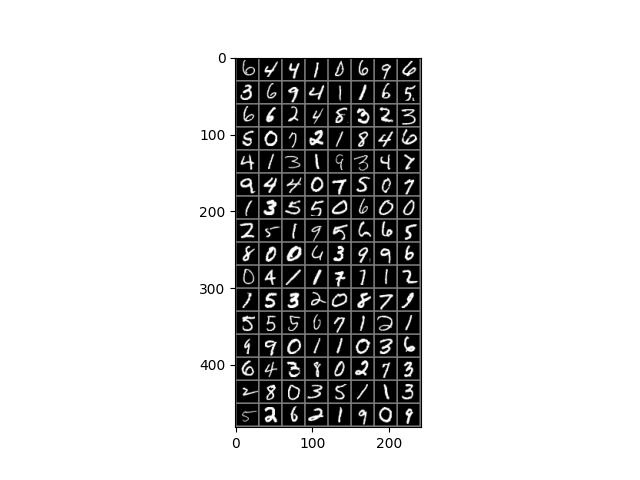
# Show images and labels
imshow(torchvision.utils.make_grid(images, nrow=8))
print("Labels:\n", labels.reshape((-1, 8)))
Labels:
 tensor([[1, 7, 9, 3, 0, 2, 8, 3],
        [6, 1, 9, 7, 8, 8, 6, 5],
        [6, 3, 1, 3, 6, 8, 4, 4],
        [2, 4, 3, 1, 4, 0, 3, 3],
        [5, 9, 4, 2, 5, 8, 6, 4],
        [3, 7, 0, 0, 2, 1, 7, 0],
        [8, 9, 9, 1, 4, 7, 0, 6],
        [5, 3, 6, 6, 7, 0, 1, 4],
        [5, 0, 9, 7, 5, 5, 9, 2],
        [9, 7, 7, 6, 1, 7, 8, 1],
        [1, 7, 2, 1, 9, 7, 6, 3],
        [0, 5, 4, 8, 1, 2, 7, 6],
        [3, 8, 8, 1, 5, 8, 6, 9],
        [8, 9, 1, 9, 4, 2, 2, 4],
        [8, 9, 4, 1, 6, 7, 2, 8],
        [9, 8, 9, 1, 1, 4, 0, 1]])
1.2. Model definition
Note that at this stage, there is nothing specific to the Akida IP. The model constructed below uses the torch.nn.Sequential module to define a standard CNN.
model_torch = torch.nn.Sequential(torch.nn.Conv2d(1, 32, 5, padding=(2, 2)),
                                  torch.nn.ReLU6(),
                                  torch.nn.MaxPool2d(kernel_size=2),
                                  torch.nn.Conv2d(32, 64, 3, stride=2),
                                  torch.nn.ReLU(),
                                  torch.nn.Dropout(0.25),
                                  torch.nn.Flatten(),
                                  torch.nn.Linear(2304, 512),
                                  torch.nn.ReLU(),
                                  torch.nn.Dropout(0.5),
                                  torch.nn.Linear(512, 10))
print(model_torch)
Sequential(
  (0): Conv2d(1, 32, kernel_size=(5, 5), stride=(1, 1), padding=(2, 2))
  (1): ReLU6()
  (2): MaxPool2d(kernel_size=2, stride=2, padding=0, dilation=1, ceil_mode=False)
  (3): Conv2d(32, 64, kernel_size=(3, 3), stride=(2, 2))
  (4): ReLU()
  (5): Dropout(p=0.25, inplace=False)
  (6): Flatten(start_dim=1, end_dim=-1)
  (7): Linear(in_features=2304, out_features=512, bias=True)
  (8): ReLU()
  (9): Dropout(p=0.5, inplace=False)
  (10): Linear(in_features=512, out_features=10, bias=True)
)
1.3. Model training
# Define training rules
optimizer = torch.optim.Adam(model_torch.parameters(), lr=1e-4)
criterion = torch.nn.CrossEntropyLoss()
epochs = 10

# Loop over the dataset multiple times
for epoch in range(epochs):
    running_loss = 0.0
    for i, data in enumerate(trainloader, 0):
        # Get the inputs and labels
        inputs, labels = data

        # Zero the parameter gradients
        optimizer.zero_grad()

        # Forward + Backward + Optimize
        outputs = model_torch(inputs)
        loss = criterion(outputs, labels)
        loss.backward()
        optimizer.step()

        # Print statistics
        running_loss += loss.detach().item()
        if (i + 1) % 100 == 0:
            print(f'[{epoch + 1}, {i + 1:5d}] loss: {running_loss / 2000:.3f}')
            running_loss = 0.0
[1,   100] loss: 0.072
[1,   200] loss: 0.025
[1,   300] loss: 0.019
[1,   400] loss: 0.016
[2,   100] loss: 0.012
[2,   200] loss: 0.011
[2,   300] loss: 0.010
[2,   400] loss: 0.008
[3,   100] loss: 0.007
[3,   200] loss: 0.007
[3,   300] loss: 0.006
[3,   400] loss: 0.006
[4,   100] loss: 0.005
[4,   200] loss: 0.005
[4,   300] loss: 0.005
[4,   400] loss: 0.005
[5,   100] loss: 0.004
[5,   200] loss: 0.004
[5,   300] loss: 0.004
[5,   400] loss: 0.004
[6,   100] loss: 0.004
[6,   200] loss: 0.003
[6,   300] loss: 0.004
[6,   400] loss: 0.003
[7,   100] loss: 0.003
[7,   200] loss: 0.003
[7,   300] loss: 0.003
[7,   400] loss: 0.003
[8,   100] loss: 0.003
[8,   200] loss: 0.003
[8,   300] loss: 0.003
[8,   400] loss: 0.003
[9,   100] loss: 0.002
[9,   200] loss: 0.003
[9,   300] loss: 0.002
[9,   400] loss: 0.003
[10,   100] loss: 0.002
[10,   200] loss: 0.002
[10,   300] loss: 0.002
[10,   400] loss: 0.003
1.4. Model testing
Evaluate the model performance on the test set. It should achieve an accuracy over 98%.
correct = 0
total = 0
with torch.no_grad():
    for data in testloader:
        inputs, labels = data
        # Calculate outputs by running images through the network
        outputs = model_torch(inputs)
        # The class with the highest score is the prediction
        _, predicted = torch.max(outputs.data, 1)
        total += labels.size(0)
        correct += (predicted == labels).sum().item()

assert correct / total >= 0.98
print(f'Test accuracy: {100 * correct // total} %')
Test accuracy: 98 %
2. Export
PyTorch models are not directly compatible with the QuantizeML quantization tool, it is therefore necessary to use an intermediate format. Like many other machine learning frameworks, PyTorch has tools to export modules in the ONNX format.
Therefore, the model is exported by the following code:
sample, _ = next(iter(trainloader))
torch.onnx.export(model_torch,
                  sample,
                  f="mnist_cnn.onnx",
                  input_names=["inputs"],
                  output_names=["outputs"],
                  dynamic_axes={'inputs': {0: 'batch_size'}, 'outputs': {0: 'batch_size'}})
============= Diagnostic Run torch.onnx.export version 2.0.1+cu118 =============
verbose: False, log level: Level.ERROR
======================= 0 NONE 0 NOTE 0 WARNING 0 ERROR ========================
Note
Find more information about how to export PyTorch models in ONNX at https://pytorch.org/docs/stable/onnx.html.
3. Quantize
An Akida accelerator processes integer activations and weights. Therefore, the floating point model must be quantized in preparation to run on an Akida accelerator.
The QuantizeML quantize()
function recognizes ModelProto objects
and can quantize them for Akida. The result is another ModelProto, compatible with the
CNN2SNN Toolkit.
Warning
ONNX and PyTorch offer their own quantization methods. You should not use those when preparing your model for Akida. Only the QuantizeML quantize() function can be used to generate a quantized model ready for conversion to Akida.
Note
For this simple model, using random samples for calibration is sufficient, as shown in the following steps.
import onnx
from quantizeml.models import quantize

# Read the exported ONNX model
model_onnx = onnx.load_model("mnist_cnn.onnx")

# Extract a batch of train samples for calibration
calib_samples = next(iter(trainloader))[0].numpy()

# Quantize
model_quantized = quantize(model_onnx, samples=calib_samples)
print(onnx.helper.printable_graph(model_quantized.graph))
Calibrating with 128/128.0 samples
graph torch_jit (
  %inputs[FLOAT, batch_sizex1x28x28]
) initializers (
  %quantize_scale[FLOAT, 1]
  %quantize_zp[UINT8, 1]
  %/0/Conv_Xpad[UINT8, 1]
  %/0/Conv_Wi[INT8, 32x1x5x5]
  %/0/Conv_B[INT32, 32]
  %/0/Conv_pads[INT64, 8]
  %/0/Conv_max_value[INT32, 1x32x1x1]
  %/0/Conv_M[UINT8, 1x32x1x1]
  %/0/Conv_S_out[FLOAT, 1x32x1x1]
  %/3/Conv_Wi[INT8, 64x32x3x3]
  %/3/Conv_B[INT32, 64]
  %/3/Conv_pads[INT64, 8]
  %/3/Conv_M[UINT8, 1x64x1x1]
  %/3/Conv_S_out[FLOAT, 1x64x1x1]
  %/7/Gemm_Wi[INT8, 512x2304]
  %/7/Gemm_B[INT32, 512]
  %/7/Gemm_M[UINT8, 1x512]
  %/7/Gemm_S_out[FLOAT, 1x512]
  %/10/Gemm_Wi[INT8, 10x512]
  %/10/Gemm_B[INT32, 10]
  %dequantizer_scale[FLOAT, 10]
) {
  %quantize = InputQuantizer[perm = [0, 1, 2, 3], scale = <Tensor>](%inputs, %quantize_scale, %quantize_zp)
  %/2/MaxPool_output_0 = QuantizedInputConv2DBiasedMaxPoolReLUClippedScaled[pool_pads = [0, 0, 0, 0], pool_size = [2, 2], pool_strides = [2, 2], scale = <Tensor>, strides = [1, 1]](%quantize, %/0/Conv_Xpad, %/0/Conv_Wi, %/0/Conv_B, %/0/Conv_pads, %/0/Conv_max_value, %/0/Conv_M, %/0/Conv_S_out)
  %/4/Relu_output_0 = QuantizedConv2DBiasedReLUScaled[scale = <Tensor>, strides = [2, 2]](%/2/MaxPool_output_0, %/3/Conv_Wi, %/3/Conv_B, %/3/Conv_pads, %/3/Conv_M, %/3/Conv_S_out)
  %/8/Relu_output_0 = QuantizedDense1DFlattenBiasedReLUScaled[scale = <Tensor>](%/4/Relu_output_0, %/7/Gemm_Wi, %/7/Gemm_B, %/7/Gemm_M, %/7/Gemm_S_out)
  %outputs = QuantizedDense1DBiased[scale = <Tensor>](%/8/Relu_output_0, %/10/Gemm_Wi, %/10/Gemm_B)
  %outputs/dequantize = Dequantizer(%outputs, %dequantizer_scale)
  return %outputs/dequantize
}
4. Convert
4.1 Convert to Akida model
The quantized model can now be converted to the native Akida format. The convert() function returns a model in Akida format ready for inference.
from cnn2snn import convert

model_akida = convert(model_quantized)
model_akida.summary()
                Model Summary
______________________________________________
Input shape  Output shape  Sequences  Layers
==============================================
[28, 28, 1]  [1, 1, 10]    1          5
______________________________________________

_________________________________________________________
Layer (type)               Output shape  Kernel shape

=========== SW//0/Conv-dequantizer (Software) ===========

/0/Conv (InputConv2D)      [14, 14, 32]  (5, 5, 1, 32)
_________________________________________________________
/3/Conv (Conv2D)           [6, 6, 64]    (3, 3, 32, 64)
_________________________________________________________
/7/Gemm (Dense1D)          [1, 1, 512]   (2304, 512)
_________________________________________________________
/10/Gemm (Dense1D)         [1, 1, 10]    (512, 10)
_________________________________________________________
dequantizer (Dequantizer)  [1, 1, 10]    N/A
_________________________________________________________
4.2. Check performance
Native PyTorch data must be presented in a different format to perform the evaluation in Akida models. Specifically:
images must be numpy-raw, with an 8-bit unsigned integer data type and
the channel dimension must be in the last dimension.
# Read raw data and convert it into numpy
x_test = testloader.dataset.data.numpy()
y_test = testloader.dataset.targets.numpy()

# Add a channel dimension to the image sets as Akida expects 4-D inputs corresponding to
# (num_samples, width, height, channels). Note: MNIST is a grayscale dataset and is unusual
# in this respect - most image data already includes a channel dimension, and this step will
# not be necessary.
x_test = x_test[..., None]
y_test = y_test[..., None]

accuracy = model_akida.evaluate(x_test, y_test)
print('Test accuracy after conversion:', accuracy)

# For non-regression purposes
assert accuracy > 0.96
Test accuracy after conversion: 0.9882000088691711
4.3 Show predictions for a single image
Display one of the test images, such as the first image in the aforementioned dataset, to visualize the output of the model.
# Test a single example
sample_image = 0
image = x_test[sample_image]
outputs = model_akida.predict(image.reshape(1, 28, 28, 1))

plt.imshow(x_test[sample_image].reshape((28, 28)), cmap="Greys")
print('Input Label:', y_test[sample_image].item())
print('Prediction Label:', outputs.squeeze().argmax())
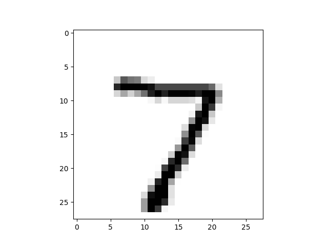
Input Label: 7
Prediction Label: 7
Total running time of the script: (2 minutes 45.263 seconds)