Advanced CNN2SNN tutorial

Warning

Please note that CNN2SNN quantization is now deprecated and shouldn’t be used anymore. QuantizeML tool replaces it. However, we wanted to keep some CNN2SNN quantization examples of use, to avoid Akida 1.0 IP based hardware support discontinuity.

This tutorial gives insights about CNN2SNN for users who want to go deeper into the quantization possibilities of Keras models. We recommend first looking at the user guide to get started with CNN2SNN.

The CNN2SNN toolkit offers an easy-to-use set of functions to get a quantized model from a native Keras model and to convert it to an Akida model compatible with the Akida NSoC. The quantize and quantize_layer high-level functions replace native Keras layers into custom CNN2SNN quantized layers which are derived from their Keras equivalents. However, these functions are not designed to choose how the weights and activations are quantized. This tutorial will present an alternative low-level method to define models with customizable quantization of weights and activations.

1. Design a CNN2SNN quantized model

Unlike the standard CNN2SNN flow where a native Keras model is quantized using the quantize and quantize_layer functions, a customizable quantized model must be directly created using quantized layers.

The CNN2SNN toolkit supplies custom quantized layers to replace native Keras neural layers (Conv2D, SeparableConv2D and Dense) and activations (ReLU).

Quantized neural layers

The CNN2SNN quantized neural layers are:

• QuantizedConv2D, derived from keras.Conv2D

• QuantizedSeparableConv2D, derived from keras.SeparableConv2D

• QuantizedDense, derived from keras.Dense

They are similar to their Keras counterparts, but have an additional argument: quantizer. This parameter expects a WeightQuantizer object that defines how the weights are discretized for a given bitwidth. Some quantizers are proposed in the CNN2SNN API:

• StdWeightQuantizer and StdPerAxisQuantizer: these two quantizers use the standard deviation of the weights to compute the range on which weights are discretized. The StdWeightQuantizer uses a range equal to a fixed number of standard deviations to discretize all weights within a layer, whereas the StdPerAxisQuantizer discretizes each feature kernel independently.

• MaxQuantizer and MaxPerAxisQuantizer: these discretize on a range based on the maximum of the absolute value of the weights. The MaxQuantizer discretizes all weights within a layer based on their global maximum, whereas the MaxPerAxisQuantizer discretizes each feature kernel, in practice the last dimension of the weights tensor, independently based on its local maximum.

If those quantizers do not fit your specific needs, you can create your own (cf. 2. Weight Quantizer Details).

Note

The QuantizedSeparableConv2D layer can accept two quantizers: one quantizer for the pointwise convolution and a quantizer_dw for the depthwise convolution. If the latter is not defined, it is set by default to the same value as quantizer.

For Akida compatibility, the depthwise quantizer must be a per-tensor quantizer (i.e. all weights within the depthwise kernel are quantized together) and not a per-axis quantizer (i.e. each feature kernel is quantized independently). See more details here.

Quantized activation layers

Similarly, a quantized activation layer returns values that are discretized on a uniform grid. Two quantized activation layers are provided to replace the native ReLU layers:

• ActivationDiscreteRelu: a linear quantizer for ReLU, clipped at value 6.

• QuantizedRelu: a configurable activation layer where max clipping value is a parameter.

It is also possible to define a custom quantized activation layer. Details are given in the section 3. Understanding quantized activation.

Note

The quantize function is a high-level helper that automatically replaces the neural layers with their corresponding quantized counterparts, using MaxPerAxisQuantizer. The ReLU layers are substituted by QuantizedRelu layers.

Create a quantized model

Here, we illustrate how to create a quantized model, equivalent to a native Keras model. We use the weight quantizers and quantized activation layers available in the CNN2SNN package. Although we present only one weight quantizer and one quantized activation, a quantized model can be a mix of any quantizers and activations. For instance, every neural layer can have a different weight quantizer with different parameters.

from tensorflow.keras import Sequential, Input, layers

# Create a native Keras toy model
model_keras = Sequential([

    # Input layer
    Input(shape=(28, 28, 1)),

    # Conv + MaxPool + BatchNorm + ReLU
    layers.Conv2D(8, 3),
    layers.MaxPool2D(),
    layers.BatchNormalization(),
    layers.ReLU(),

    # Flatten + Dense + Softmax
    layers.Flatten(),
    layers.Dense(10),
    layers.Softmax()
])

model_keras.summary()

Model: "sequential_20"
_________________________________________________________________
 Layer (type)                Output Shape              Param #
=================================================================
 conv2d_1 (Conv2D)           (None, 26, 26, 8)         80

 max_pooling2d (MaxPooling2  (None, 13, 13, 8)         0
 D)

 batch_normalization_1 (Bat  (None, 13, 13, 8)         32
 chNormalization)

 re_lu_1 (ReLU)              (None, 13, 13, 8)         0

 flatten_1 (Flatten)         (None, 1352)              0

 dense_1 (Dense)             (None, 10)                13530

 softmax (Softmax)           (None, 10)                0

=================================================================
Total params: 13642 (53.29 KB)
Trainable params: 13626 (53.23 KB)
Non-trainable params: 16 (64.00 Byte)
_________________________________________________________________

from cnn2snn import quantization_layers as qlayers
from cnn2snn import quantization_ops as qops

# Prepare weight quantizers
q1 = qops.MaxQuantizer(bitwidth=8)
q2 = qops.MaxQuantizer(bitwidth=4)

# Get layer names to set them in the quantized model
names = [layer.name for layer in model_keras.layers]

# Create a quantized model, equivalent to the native Keras model
model_quantized = Sequential([

    # Input layer
    Input(shape=(28, 28, 1)),

    # Conv + MaxPool + BatchNorm + ReLU
    qlayers.QuantizedConv2D(8, 3, quantizer=q1, name=names[0]),
    layers.MaxPool2D(name=names[1]),
    layers.BatchNormalization(name=names[2]),
    qlayers.QuantizedReLU(bitwidth=4, name=names[3]),

    # Flatten + Dense + Softmax
    layers.Flatten(name=names[4]),
    qlayers.QuantizedDense(10, quantizer=q2, name=names[5]),
    layers.Softmax(name=names[6]),
])

model_quantized.summary()

Model: "sequential_21"
_________________________________________________________________
 Layer (type)                Output Shape              Param #
=================================================================
 conv2d_1 (QuantizedConv2D)  (None, 26, 26, 8)         80

 max_pooling2d (MaxPooling2  (None, 13, 13, 8)         0
 D)

 batch_normalization_1 (Bat  (None, 13, 13, 8)         32
 chNormalization)

 re_lu_1 (QuantizedReLU)     (None, 13, 13, 8)         0

 flatten_1 (Flatten)         (None, 1352)              0

 dense_1 (QuantizedDense)    (None, 10)                13530

 softmax (Softmax)           (None, 10)                0

=================================================================
Total params: 13642 (53.29 KB)
Trainable params: 13626 (53.23 KB)
Non-trainable params: 16 (64.00 Byte)
_________________________________________________________________

2. Weight Quantizer Details

How a weight quantizer works

The purpose of a weight quantizer is to compute a tensor of discretized weights. It can be split into two operations:

• an optional transformation applied on the weights, e.g. a shift, a non-linear transformation, …

• the quantization of the weights.

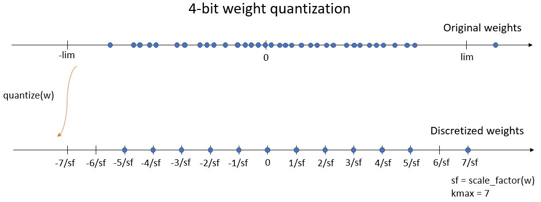
For Akida compatibility, the weights must be discretized on a symmetric grid defined by two parameters:

• the bitwidth defines the number of unique values the weights can take. We define kmax = 2^(bitwidth-1) - 1, being the maximum integer value of the symmetric quantization scheme. For instance, a 4-bit quantizer must return weights on a grid of 15 values, between -7 and 7. Here, kmax = 7.

• the symmetric range on which the weights will be discretized (let’s say between -lim and lim). Instead of working with the range, we use the scale factor which is defined by sf = kmax / lim, where sf is the scale factor. For instance with a 4-bit quantizer, the discretized weights will be on the grid [-7/sf, -6/sf, …, -1/sf, 0, 1/sf, …, 6/sf, 7/sf]. The maximum discrete value 7/sf is equal to lim, the limit of the range (see figure below).

When training, the weight quantization is applied during the forward pass: the weights are quantized and then used for the convolution or the fully connected operation. However, during the back-propagation phase, the gradient is computed as if there were no quantization and the weights are updated based on their original values before quantization. This is usually called the “Straight-Through Estimator” (STE) and it can be done using the tf.stop_gradient function.

Note

Remember that the weights are stored as standard float values in the model. To get the quantized weights, you must first retrieve the standard weights, using get_weights(). Then, you can apply the quantize function of the weight quantizer to obtain the discretized weights. Finally, if you want to get the integer quantized values (between -kmax and kmax), you must multiply the discretized weights by the scale factor.

How to create a custom weight quantizer

The CNN2SNN API proposes a way to create a custom weight quantizer. It must be derived from the WeightQuantizer base class and must override two methods:

• the scale_factor(w) method, returning the scale factor based on the input weights. The output must be a scalar or vectorial TensorFlow tensor. Per-tensor quantization will give a single scalar value, whereas per-axis quantization will yield a vector with a scale factor for each feature kernel.

• the quantize(w) method, returning the discretized weights based on the scale factor and the bitwidth. A Tensorflow tensor must be returned. The two operations (optional transformation and quantization) are performed in here.

Note

To be able to correctly train a quantized model, it is important to implement the STE estimator in the quantize function, by using tf.stop_gradient at the quantization operation.

If there is no need for the optional transformation in the custom quantizer, the CNN2SNN toolkit gives a LinearWeightQuantizer that skips this step. The quantize function is already provided and only the scale_factor function must be overridden.

Why use a different quantizer

Let’s now see a use case where it is interesting to consider the behaviour of different quantizers. The MaxQuantizer used in the QuantizedDense layer of our above model discretizes the weights based on their maximum value. The default MaxPerAxisQuantizer has a similar behaviour with an additional per-axis quantization design. If weights contain outliers, that are very large weights in absolute value, this quantization scheme based on maximum value can be inappropriate. Let’s look at it in practice: we retrieve the weights of the QuantizedDense layer and compute the discretized counterparts using the MaxQuantizer of the layer.

import numpy as np
import tensorflow as tf
import matplotlib.pyplot as plt

# Retrieve weights and quantizer of the QuantizedDense layer
dense_name = names[5]
quantizer = model_quantized.get_layer(dense_name).quantizer
w = model_quantized.get_layer(dense_name).get_weights()[0]

# Artificially add outliers
w[:5, :] = 0.5

# Compute discretized weights
wq = quantizer.quantize(tf.constant(w)).numpy()


# Show original and discretized weights histograms
def plot_discretized_weights(w, wq):
    xlim = [-0.095, 0.53]
    fig, (ax1, ax2) = plt.subplots(1, 2)
    ax1.hist(w.flatten(), bins=50)
    ax1.set_xlim(xlim)
    ax1.get_yaxis().set_visible(False)
    ax1.title.set_text("Original weights distribution")

    vals, counts = np.unique(wq, return_counts=True)
    ax2.bar(vals, counts, 0.005)
    ax2.set_xlim(xlim)
    ax2.get_yaxis().set_visible(False)
    ax2.title.set_text("Discretized weights distribution")

    plt.tight_layout()
    plt.show()


plot_discretized_weights(w, wq)

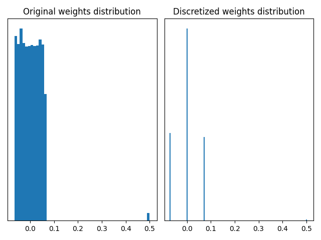
The graphs above illustrate that a MaxQuantizer applied on weights with outliers will keep the full range of weights to discretize. In this use case, the large majority of weights is between -0.1 and 0.1, and are discretized on only three quantization values. The outliers at 0.5 are preserved after quantization. If outlier weights don’t represent much information in the layer, it can be preferable to use another weight quantizer which “forgets” them.

The StdWeightQuantizer is a good alternative for this use case: the quantization range is based on the standard deviation of the original weights. Outliers have little impact on the standard deviation of the weights. Then the outliers can be out of the range based on the standard deviation.

In this tutorial, instead of directly using the StdWeightQuantizer, we present how to create a quantizer. The custom quantizer created below is a simplified version of the StdWeightQuantizer. It is derived from the LinearWeightQuantizer. As mentioned above, the quantize function is already implemented in LinearWeightQuantizer. Only the scale_factor function must be overridden.

# Define a custom weight quantizer
class CustomStdQuantizer(qops.LinearWeightQuantizer):
    """This is a custom weight quantizer that defines the scale factor based
    on the standard deviation of the weights.

    The weights in range (-2*std, 2*std) are quantized into (2**bitwidth - 1)
    levels and the weights outside this range are clipped to ±2*std.
    """

    def scale_factor(self, w):
        std_dev = tf.math.reduce_std(w)
        return self.kmax_ / (2 * std_dev)


quantizer_std = CustomStdQuantizer(bitwidth=4)

# Compute discretized weights
wq = quantizer_std.quantize(tf.constant(w)).numpy()

# Show original and discretized weights histograms
plot_discretized_weights(w, wq)

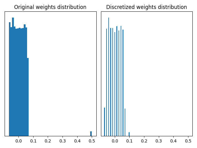
The two graphs above show that using a quantizer based on the standard deviation can remove the outliers and give a finer discretization of the weights between -0.1 and 0.1. In this toy example, the MaxQuantizer discretizes the “small” weights on 3 quantization values, whereas the CustomStdQuantizer discretizes them on about 13-14 quantization values. Depending on the need to preserve the outliers or not, one quantizer or the other is preferable.

In our experience, the MaxPerAxisQuantizer yields better results in most use cases, especially for post-training quantization, which is why it is the default quantizer.

3. Understanding quantized activation

A quantized activation layer works as a ReLU layer with an additional quantization step. It can then be seen as a succession of two operations:

• a linear activation function, clipped between zero and a maximum activation value

• the quantization, which is a ceiling operation. The activations will be uniformly quantized between zero and the maximum activation value.

The linear activation function is defined by (cf. the blue line in the graph below):

• the activation threshold: the value above which a neuron fires

• the maximum activation value: any activation above will be clipped

The quantization operation is defined by one parameter: the bitwidth. The activation function is quantized using the ceiling operator on 2^bitwidth - 1 positive activation levels. For instance, a 4-bit quantized activation gives 15 activation levels (plus the zero activation) uniformly distributed between zero and the maximum activation value (cf. the orange line in the graph).

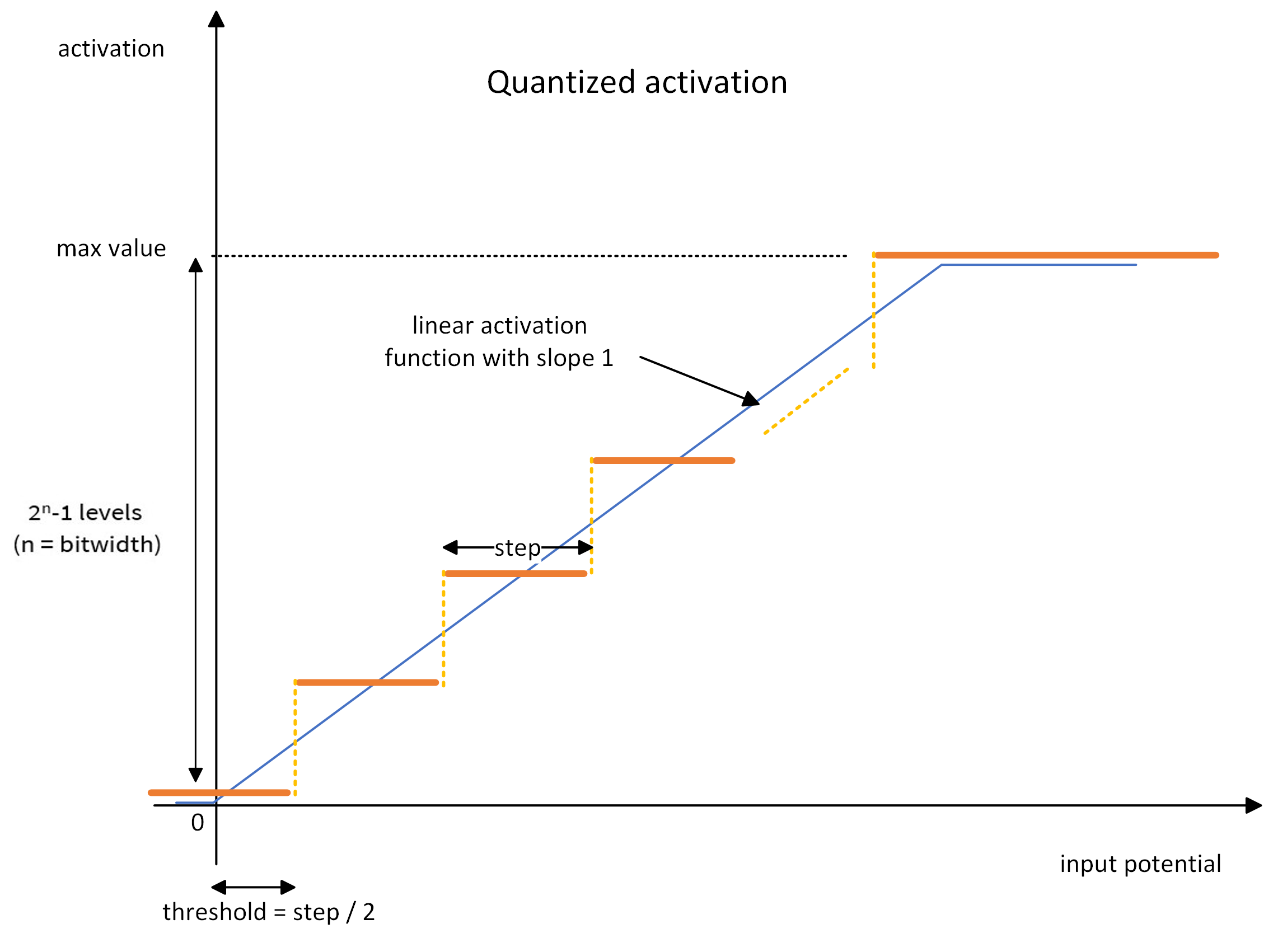
During training, the ceiling quantization is performed in the forward pass: the activations are discretized and then transferred to the next layer. However, during the back-propagation phase, the gradient is computed as if there were no quantization: only the gradient of the clipped linear activation function (blue line above) is back-propagated. Like for weight quantizers, this STE estimator is done using the tf.stop_gradient function.

4. How to deal with too high scale factors

A quantized Keras model may have sometimes very high scale factors, i.e. very small weights, in the neural layers. During conversion into an Akida model, these scale factors are used to compute the Akida fire thresholds and steps required for Akida inference. However, these fire thresholds and steps are limited in memory on NSoC. It may happen that their values are too big to fit into memory and then a Runtime Error occurs at Akida inference, e.g. Runtime Error: Error when programming layer 'separable_8': Backend Hardware(CNP): 1246278 cannot fit in a 20-bit unsigned integer.

If you’re facing this issue, it is necessary to retrain your Keras model to avoid too high scale factors in the neural layers. One possible reason for these high scale factors is the presence of very small gammas in BatchNormalization (BN) layers. Indeed, when folding BN layers into their preceding neural layers, the weights corresponding to tiny BN gammas become in turn very small, which leads to high scale factors. The akida_models package provides a tool to add constraint on BN gammas: the gammas are clipped to a minimum value of 1e-2: the gammas cannot be smaller than this threshold. The code snippet below illustrates how to use the provided tool. Note that it must be applied on the Keras float (or quantized) model before folding BN layers.

from akida_models.gamma_constraint import add_gamma_constraint

# Add BN gamma constraint on all BN layers of the model
model_keras_with_gamma_constraint = add_gamma_constraint(model_keras)

The new model can then be trained using compile() and fit() and quantized if needed. The trained model will not have BN gammas less than 1e-2, which is valuable to avoid very high scale factors.