Note
Go to the end to download the full example code.
Tips to set Akida edge learning parameters
Important
Edge learning is only supported for Akida 1.0 models and devices.
This tutorial gives details about the Akida learning parameters and tips to set their values in a first try in an edge learning application. The KWS dataset and the DS-CNN-edge model are used as a classification example to showcase the handy tips.
One can consult the KWS edge learning tutorial for a first approach about Akida learning.
Note
The hints given in this tutorial are not a promise to get the best performance. They can be seen as an initialization, before fine-tuning. Besides, even if these tips provide good estimates in most examples, they can’t be guaranteed to work for every application.
1. Akida learning parameters
To be ready for learning, an Akida model must be composed of:
a feature extractor returning binary spikes: this part is usually trained using the CNN2SNN toolkit.
an Akida trainable layer added on top of the feature extractor: it must have 1-bit weights and several output neurons per class.
The last trainable layer must be correctly configured to get good learning performance. The two main parameters to set are:
the number of weights
the number of neurons per class
In the next sections, details about these hyper-parameters are given with handy tips to give a first estimation.
2. Create Akida model
In a first stage, we will create the Akida feature extractor returning binary spikes. From then, we will be able to estimate the parameters for the trainable layer that will be added later.
After loading the KWS dataset, we create the pre-trained TF-Keras model and convert it to an Akida model. We then remove the last layer to get the feature extractor.
from akida import Model, InputData, FullyConnected

import pickle

from akida_models import fetch_file

# Fetch pre-processed data for 32 keywords
fname = fetch_file(
    fname='kws_preprocessed_all_words_except_backward_follow_forward.pkl',
    origin="https://data.brainchip.com/dataset-mirror/kws/kws_preprocessed_all_words_except_backward_follow_forward.pkl",
    cache_subdir='datasets/kws')
with open(fname, 'rb') as f:
    [x_train, y_train, _, _, _, _, word_to_index, _] = pickle.load(f)
Note
Edge learning is only supported for Akida 1.0 models for now.
from cnn2snn import convert, set_akida_version, AkidaVersion
from akida_models import ds_cnn_kws_pretrained

# Instantiate a quantized model with pretrained quantized weights
with set_akida_version(AkidaVersion.v1):
    model = ds_cnn_kws_pretrained()

# Convert to an Akida model
model_ak = convert(model)

# Remove last layer
model_ak.pop_layer()
model_ak.summary()
/usr/local/lib/python3.11/dist-packages/akida_models/model_io.py:147: UserWarning: Model ds_cnn_kws_iq8_wq4_aq4_laq1.h5 has been trained with akida_models 1.1.10 which is the last version supporting 1.0 models training. Continuing execution.
  warnings.warn(f'Model {model_name_v1} has been trained with akida_models 1.1.10 which is '
                Model Summary
______________________________________________
Input shape  Output shape  Sequences  Layers
==============================================
[49, 10, 1]  [1, 1, 64]    1          5
______________________________________________

_______________________________________________________
Layer (type)             Output shape  Kernel shape

=========== SW/conv_0-separable_4 (Software) ==========

conv_0 (InputConv.)      [25, 5, 64]   (5, 5, 1, 64)
_______________________________________________________
separable_1 (Sep.Conv.)  [25, 5, 64]   (3, 3, 64, 1)
_______________________________________________________
                                       (1, 1, 64, 64)
_______________________________________________________
separable_2 (Sep.Conv.)  [25, 5, 64]   (3, 3, 64, 1)
_______________________________________________________
                                       (1, 1, 64, 64)
_______________________________________________________
separable_3 (Sep.Conv.)  [25, 5, 64]   (3, 3, 64, 1)
_______________________________________________________
                                       (1, 1, 64, 64)
_______________________________________________________
separable_4 (Sep.Conv.)  [1, 1, 64]    (3, 3, 64, 1)
_______________________________________________________
                                       (1, 1, 64, 64)
_______________________________________________________
3. Estimate the required number of weights of the trainable layer
The number of weights corresponds to the number of connections for each neuron. The smaller the number of weights, the less specific the neurons will be. Setting this parameter correctly is important.
Although the last trainable layer hasn’t been created yet, we can already estimate the number of weights. This estimation is based on the statistics of the output spikes from the feature extractor. Intuitively, a sample producing N spikes at the end of the feature extractor could be perfectly represented with a neuron with N weights. We then use the median of the number of output spikes for all samples.
To reduce computing time, using only a subset of the whole dataset may be sufficient to get an estimation of the number of spikes. We then set the number of weights to a value slightly higher than the median of the number of spikes: we generally choose 1.2 x median of number of spikes, which seems to give good results.
For a deeper analysis of the output spikes from the feature extractor, one could look at the distribution of the number of spikes, either for all samples or for samples of each class separately. This analysis is not shown here.
import numpy as np

# Forward samples to get the number of output spikes
# Here, 10% of the training set is sufficient for a good estimation
num_samples_to_use = int(len(x_train) / 10)
spikes = model_ak.forward(x_train[:num_samples_to_use])

# Compute the median of the number of output spikes
median_spikes = np.median(spikes.sum(axis=(1, 2, 3)))
print(f"Median of number of spikes: {median_spikes}")

# Set the number of weights to 1.2 x median
num_weights = int(1.2 * median_spikes)
print(f"The number of weights is then set to: {num_weights}")
Median of number of spikes: 23.0
The number of weights is then set to: 27
4. Estimate the number of neurons per class
Unlike a standard CNN network where each class is represented by a single output neuron, an Akida native training requires several neurons for each class to better represent the class variability. Choosing the right number of neurons per class is a trade-off between enough neurons to represent the classes’ variabilities, but not too many neurons implying more memory and computing time. This is similar to clustering algorithms where the clusters represent the distribution of the data. Note that, like clustering algorithms, this analysis requires to have more samples per class than the number of neurons per class: only one neuron can learn per sample. Having more neurons than samples, the extra neurons are guaranteed to be wasted.
One direct option is to train the classification layer using the whole dataset with different values of number of neurons per class. Looking at the validation accuracy, it should increase with more neurons per class, then reach a plateau where adding more neurons has very small effect. Choosing the value where the accuracy begins to flatten is a good estimation.
However, this method is very time consuming since it requires multiple trainings using the whole dataset. Another option is to only train on a few number of classes. Rather than measuring accuracy, we measure the error between the potential of the matching neuron and the maximum theoretical potential. Taking a simple example:
Let’s say 3 neurons per class, with 180 weights
A sample of a given class returns 3 potentials for the 3 neurons of its class: [12, 153, 97]. The maximum potential is 153.
The error between the sample and the neuron is 180 - 153 = 27.
Compute the loss being the sum of the errors for all samples of a class.
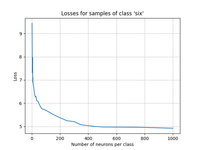
Visualizing the loss for a given class as a function of the number of neurons gives hints to have a first estimation of the number of neurons per class. Visualizing the number of neurons that have learned as a function of the number of neurons per class provides a similar analysis.
In this tutorial, we only present this analysis for one class (word ‘six’).
from akida import AkidaUnsupervised


def compute_losses(model,
                   samples,
                   neurons_per_class,
                   num_weights,
                   learning_competition=0.1,
                   num_repetitions=1):
    """Compute losses after training an Akida FullyConnected layer for samples
    of one class.

    For each value of 'neurons_per_class', a training is performed, and the loss
    and the number of neurons that have learned are returned.

    Args:
        model: an Akida model for feature extraction
        samples: a NumPy array of input samples of one class
        neurons_per_class: an 1-D iterable object storing the integer values of
            the number of neurons to test
        num_weights: the number of non-zero weights in each neuron
        learning_competition: the learning competition of the trainable layer
        num_repetitions: the number of times the training must be performed.
            The training with the minimum loss will be kept.

    Returns:
        the losses and the numbers of neurons that have learned

    """
    spikes = model.forward(samples)

    def create_one_fc_model(units):
        model_fc = Model()
        model_fc.add(
            InputData(name="input",
                      input_shape=(1, 1, spikes.shape[-1]),
                      input_bits=1))
        layer_fc = FullyConnected(name='akida_edge_layer',
                                  units=units,
                                  activation=False)
        model_fc.add(layer_fc)
        model_fc.compile(optimizer=AkidaUnsupervised(num_weights=num_weights,
                                                     learning_competition=learning_competition))
        return model_fc

    losses = np.zeros((len(neurons_per_class), num_repetitions))
    num_learned_neurons = np.zeros((len(neurons_per_class), num_repetitions))
    for idx, n in enumerate(neurons_per_class):
        for i in range(num_repetitions):
            model_fc = create_one_fc_model(units=n)

            # Train model
            permut_spikes = np.random.permutation(spikes)
            model_fc.fit(permut_spikes)

            # Get max potentials
            max_potentials = model_fc.forward(permut_spikes).max(axis=-1)
            losses[idx, i] = np.sum(num_weights - max_potentials)

            # Get threshold learning
            th_learn = model_fc.get_layer('akida_edge_layer').get_variable(
                'threshold_learning')
            num_learned_neurons[idx, i] = np.sum(th_learn > 0)

    return losses.min(axis=1) / len(spikes), num_learned_neurons.min(axis=1)
# Choose a word to analyze and the values for the number of neurons
word = 'six'
neurons_per_class = [
    2, 3, 4, 5, 6, 7, 8, 9, 10, 15, 20, 25, 30, 35, 40, 45, 50, 60, 70, 80, 90,
    100, 150, 200, 250, 300, 350, 400, 450, 500, 750, 1000
]

# Compute the losses for word 'six' and different number of neurons
idx_samples = (y_train == word_to_index[word])
x_train_word = x_train[idx_samples]
losses, num_learned_neurons = compute_losses(model_ak, x_train_word,
                                             neurons_per_class, num_weights)
import matplotlib.pyplot as plt

plt.plot(np.array(neurons_per_class), losses)
plt.xlabel("Number of neurons per class")
plt.ylabel("Loss")
plt.title(f"Losses for samples of class '{word}'")
plt.grid(linestyle='--')
plt.show()
plt.plot(np.array(neurons_per_class), num_learned_neurons)
plt.xlabel("Number of neurons per class")
plt.ylabel("Nb of neurons that have learned")
plt.title(f"Nb of neurons that have learned for samples of class '{word}'")
plt.grid(linestyle='--')
plt.show()
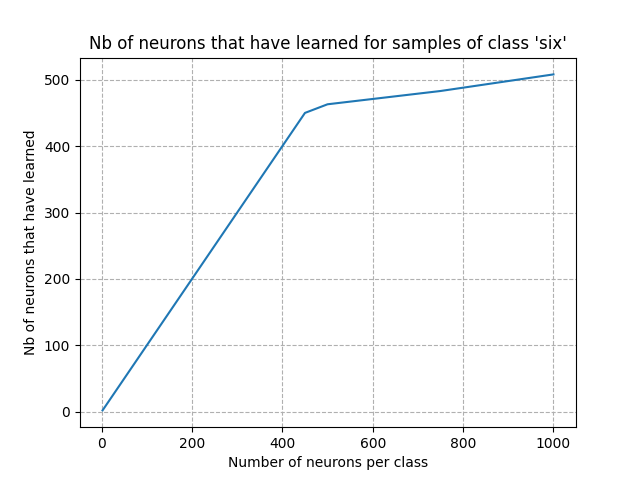
From the figures above, we can see that the point of inflection occurred with about 300 neurons. Setting the number of neurons per class to this value is a good starting point: we expect a very good accuracy after training. Adding more neurons won’t improve the accuracy and will increase the computing time.
However, one could gradually reduce the number of neurons per class to see its influence on the accuracy of a complete training. In the KWS edge tutorial, we finally set this value to 50 because it is a good trade-off between computing time and our target accuracy. The table below presents the validation accuracy after training for different numbers of neurons. We can see that there is no increase for a number of neurons per class higher than 300. Note that in this use case, the validation accuracy remains very high even for a small number of neurons per class: one should be aware that this small decrease in accuracy cannot be generalized for all use cases.
Nb. neurons |
Accuracy |
Time ratio |
|---|---|---|
10 |
91.6 % |
0.83 |
20 |
91.8 % |
0.84 |
50 |
92.1 % |
0.86 |
100 |
92.3 % |
0.89 |
200 |
92.5 % |
0.94 |
300 |
92.6 % |
1 |
400 |
92.5 % |
1.05 |
500 |
92.5 % |
1.10 |
Total running time of the script: (0 minutes 6.975 seconds)